Fill up the tank - Challenge 1: Varying the initial water level
Task
Study how the water level in the tank behaves for different values of the starting level  . What do you expect? Consider the values
  , while keeping the other parameters the same.

Figure 1: Water level in the tank for the considered values of .
This figure reports how the water level  varies according to different values of . What we can observe from the obtained graphs is that changing the initial water level modifies the initial behavior, which can be increasing or decreasing.
However, if we wait enough time, the level will reach some equilibrium value  , i.e. the water level reaches this value and no longer changes.
We recall that the equation describing how the water level changes in the tank is:

where is the water level in the tank at time  ,
,  is the area of the base of the tank,
  is the volumetric inflow, and
 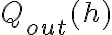 the volumetric outflow.
We can write  , where
  is the cross-section area of the outlet and
  is the velocity of the water exiting the tank. Using Torricelli’s law
  , we obtain:
 .
.
Moreover, we assume that the initial water level at time  is
is 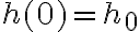 .
.
We can use the Euler method to find the discrete approximation of :
![h_{n+1} = h_n + \frac{\Delta t}{A_t} \big[\, Q_{in} - A_{out} \sqrt{2 g h_n} \,\big]](https://pok.kdevs.it/filter/tex/pix.php/e7498a4fc5b7747fb76d082666002700.gif "h_{n+1} = h_n + \frac{\Delta t}{A_t} \big[\, Q_{in} - A_{out} \sqrt{2 g h_n} \,\big]") , for
, for 
Here  is our numerical approximation of
  . Starting from different values of , we can then compute
  by recursively using this equation.
We can also notice that is independent of the specific initial value . The equilibrium value that we observe depends directly on the inflow value: at equilibrium we have  (because
  is not changing anymore), i.e.
 ,
,
which yields:
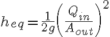 .
.
You can also verify this expression by comparing it with the final value  obtained from the numerical simulation.
To test different values of , we can enclose the code that we previously used in a for loop. Up to now, we have used the loop syntax in the form:
for i in range(N):
The expression range(N) implicitly generates all integers from  to
to  , assigning each value to the variable
 i at every iteration. However, we can pass a custom list of values. For example:
for h_0 in [0, 1, 2, 5, 8]:
In this way, the variable automatically takes on the values we want to test for the initial water level. At each iteration, we compute the numerical solution for that choice of and plot it. To label each curve we pass a string to the label argument in plt.plot(), and finally create a legend with plt.legend(). The final Python code for the solution is the following:
import matplotlib.pyplot as plt  # import package for plot

# Physical parameters
Q_in = 1.0      # inflow rate
A_t = 1.0       # tank cross-sectional area (m^2)
A_out = 0.1     # outlet area (m^2)
g = 9.81        # gravity

# Simulation time parameters
T = 100         # total simulation time
N = 1000        # number of time steps
dt = T / N      # time step

# outflow rate Q_out
def Q_out(h):
    return A_out * (2 * g * h) ** 0.5

plt.figure(figsize=(10, 5))

# loop over different values of initial water level
for h0 in [0, 2, 5, 8, 10]:

    # lists to store the solution
    times = [0.0] * (N + 1)
    h = [0.0] * (N + 1)
    h[0] = h0

    for i in range(N):
        dh = dt * (Q_in - Q_out(h[i]))
        h[i + 1] = h[i] + dh
        times[i + 1] = (i + 1) * dt

    plt.plot(times, h, label="h0 = " + str(h0))

plt.xlabel("Time (s)")
plt.ylabel("Water level (m)")
plt.title("Water level over time for different h0")
plt.legend()
plt.grid()
plt.show()
To test different values of , we can enclose the code that we previously used in a for loop. Up to now, we have used the for syntax in this way:
for i = 1:N
    % Instructions ...
end
Implicitly, the syntax 1:N generates a vector containing all integer numbers between  and
and  , and at each new iteration the variable
 i takes the next value in this vector. However, we can also use a custom vector such as:
for h_0 = [0, 1, 2, 5, 8]
    % Instructions ...
end
In this way, automatically assumes the values that we want to test for the initial water level. We can then save each result in a vector and plot them. To this aim, we create an empty plot with figure(), then we use the keyword hold on to specify that we want to plot all the graphs in the same figure. Finally, we can use legend() to assign a different label to each graph. The final Matlab code for the solution is the following:
% Function to define the inflow rate
Q_in = @(t) 1;

% Function to calculate the outflow rate based on the water level and outlet area
Q_out = @(A_out, h) sqrt(2 * 9.81 * max(h, 0)) * A_out;

A_out = 0.1;  % outlet area (m^2)
A_t   = 1;    % tank cross-sectional area (m^2)

% Simulation time parameters
T  = 100;     % total simulation time (s)
N  = 1000;    % number of time steps
dt = T / N;   % time step

% Create figure for plotting
figure();
grid on();
hold on();

% Loop over different initial water levels
for h0 = [0, 1, 2, 5, 8]

    % Arrays to store data for plotting
    times = zeros(1, N + 1);
    h     = zeros(1, N + 1);
    h(1)  = h0;
    t     = 0;

    % Simulate the water level over time
    for i = 1:N
        t = t + dt;
        h(i + 1) = h(i) + (Q_in(t) - Q_out(A_out, h(i))) * dt;
        times(i + 1) = t;
    end

    plot(times, h, '-');
end

legend('h0 = 0', 'h0 = 1', 'h0 = 2', 'h0 = 5', 'h0 = 8');