Fill up the tank - Challenge 3: Non-constant water inflow
Task
Up to now, we considered a constant inflow 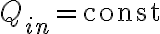 , i.e. the speed at which water enters the tank does not change over time. How can you modify the code to account for an inflow that is a function of time? Try to simulate the water level for three different inflow functions:
 ,
,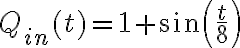 ,
,
The figure shows the solution (water level in the tank) obtained using different inflow function  .
.

Figure 1: Water level in the tank for the different expressions of  considered.
Unsurprisingly, when the inflow oscillates in time like a sine wave, the water level in the tank behaves sinusoidally too. What is more surprising is that even though the two sine waves that we used have the same amplitude and differ only by frequency, the amplitude of the oscillations in water level are very different in the two cases. In regard to the piecewise constant inflow case, we can see that the water level evolution changes abruptly at  : for
: for  the level rises until it almost reaches an equilibrium, then for
  it starts decreasing, asymptotically reaching a new, lower equilibrium value.
Our approximating equation becomes:
![h_{n+1} = h_n + \frac{\Delta t}{A_t} \big[\, Q_{in}(t_n) - A_{out} \sqrt{2 g h_n} \,\big]](https://pok.kdevs.it/filter/tex/pix.php/17b8239f8179ce60e1a0a7731c0e3383.gif "h_{n+1} = h_n + \frac{\Delta t}{A_t} \big[\, Q_{in}(t_n) - A_{out} \sqrt{2 g h_n} \,\big]") , for
, for  .
.
where to account for non constant inflow, we just substitute for 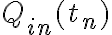 , recalling that
 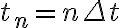 .
.
Since the water inflow is prescribed as a function of time, we can model it in our code with a corresponding function. The syntax for function definition in Python goes like this:
def Q_in1(t):
    return 1 + sin(t/4)
However, there is an alternative way that uses lambda functions. The lambda keyword (which takes its name from lambda calculus) can be used to quickly define a function object:
Q_in1 = lambda t: 1 + sin(t/4)
Defining a piecewise function is trickier, but we can do it by employing Boolean expressions. We can then define the piecewise function that we need as follows:
Q_in3 = lambda t: 1.5*(t <= 50) + 0.5*(t > 50)
The Boolean expression (t <= 50) returns 1 if t is less or equal than 50 (in other words when t <= 50 is true), otherwise (i.e. when t <= 50 is false) it returns 0.
Employing lambda functions allows us to put them in lists and use a "trick" with for loops to easily loop over different functions.
for Q_in in [Q_in1, Q_in2, Q_in3]:
    # instructions ...
The full Python code for the solution is as follows:
import matplotlib.pyplot as plt  # import package for plot
from math import sin             # import for sine function

# Physical parameters
A_t = 1       # tank cross-sectional area (m^2)
A_out = 0.1   # outlet area (m^2)
g = 9.81      # gravity
h0 = 1        # initial water level

# Simulation time parameters
T = 100       # total simulation time
N = 1000      # number of time steps
dt = T / N    # time step

# outflow rate Q_out
Q_out = lambda h: A_out * (2 * g * max(0, h)) ** 0.5

# inflow rate
Q_in1 = lambda t: 1 + sin(t / 4)
Q_in2 = lambda t: 1 + sin(t / 8)
Q_in3 = lambda t: 1.5 * (t <= 50) + 0.5 * (t > 50)
labels = ['1+ sin(t/4)', '1+ sin(t/8)', 'Piecewise constant']  # labels for the legend

plt.figure(figsize=(10, 5))

# loop over different inflow functions
for j, Q_in in enumerate([Q_in1, Q_in2, Q_in3]):

    # lists to store the solution
    times = (N + 1) * [0]
    h = (N + 1) * [0]
    h[0] = h0

    for i in range(N):
        dh = dt * (Q_in(i * dt) - Q_out(h[i]))
        h[i + 1] = h[i] + dh
        times[i + 1] = (i + 1) * dt

    plt.plot(times, h, label=labels[j])

plt.xlabel("Time (s)")
plt.ylabel("Water Level (m)")
plt.title("Water Level Over Time for Different Q_in")
plt.legend()
plt.grid()
plt.show()
Since the water inflow is prescribed as a function of time, we can model it in our code with a corresponding function. In Matlab, we can use anonymous functions, also known as function handles, for this purpose. Anonymous functions enable easy definition of mathematical functions using the following syntax:
Q_in1 = @(t) 1 + sin(t/4);
Defining a piecewise function is trickier, but we can do it by employing Boolean expressions. We can then define the piecewise function that we need as follows:
Q_in3 = @(t) 1.5*(t <= 50) + 0.5*(t > 50);
The Boolean expression (t <= 50) returns 1 if t is less or equal than 50 (in other words when t <= 50 is true), otherwise (i.e. when t <= 50 is false) it returns 0.
Anonymous functions cannot be inserted into vectors, which are reserved for real or complex numbers. However, Matlab provides a more general data structure that can contain any Matlab object, called cell arrays. A cell array is created and accessed using curly braces {}:
my_cell_array = {Q_in1, Q_in2, Q_in3};
Q_in = my_cell_array{1}; % Get the first element of the cell array
Cell arrays are useful, for example, to store vectors of different lengths in a single list. In this case, we can use one to easily loop over the functions we need to test:
for i = 1:3
    Q_in = my_cell_array{i};
    % Instructions ...
end
The full Matlab code for the solution is as follows:
% Function to calculate the outflow rate based on the water level and outlet area
Q_out = @(A_out, h) sqrt(2 * 9.81 * max(h, 0)) * A_out;
A_out = 0.1;   % Outlet area (m^2)
A_t   = 1;     % Tank cross-sectional area (m^2)

% Simulation time parameters
T = 100;       % Total simulation time (seconds)
N = 1000;      % Number of time steps
% Calculate the time step size
dt = T / N;

% Functions to define the inflow rate function
Q_in1 = @(t) 1 + sin(t/4);
Q_in2 = @(t) 1 + sin(t/8);
Q_in3 = @(t) 1.5 * (t <= 50) + 0.5 * (t > 50);
inflows = {Q_in1, Q_in2, Q_in3};

% Create figure for plotting
figure();
grid on;
hold on;

% Loop over different inflow functions
for i = 1:3
    Q_in = inflows{i};

    % Create arrays to store data for plotting
    times = zeros(1, N + 1);
    h     = zeros(1, N + 1);
    h(1)  = h0;
    t     = 0;

    % Simulate the water level over time
    for i = 1:N
        t = t + dt;
        h(i + 1) = h(i) + (Q_in(t) - Q_out(A_out, h(i))) * dt;
        times(i + 1) = t;
    end

    plot(times, h, '-');
end

legend('1+ sin(t/4)', '1+ sin(t/8)', 'Piecewise constant');