Computational Science & Computational Learning with Python and MATLAB: Predict wildfire risk - Challenge 1: Using the Buildup Index

Task

Perform linear regression between the Buildup Index (BUI) and the Fire Weather Index (FWI) in the Algerian Forest Dataset.

The figure shows the dataset and the corresponding regression line.

Figure 1: BUI-FWI dataset points in blue, and corresponding regression line in red.

We can see from the value of the regression line slope $m = 0.3353$ and from the graph in Figure 1 that the correlation between BUI and FWI is positive. This is unsurprising: the Buildup Index measures the amount of fuel available in the environment, so higher BUI means that fires spread more easily once they start, corresponding to higher fire risk.

We want to model the relation between an independent variable $x$ and a dependent variable $y$ with a line of the form:

$y = m x + q,$

where $m$ is the slope of the line and $q$ is its y-intercept.

To find the best-fitting line, we use the method of least squares, which minimizes the sum of squared residuals, i.e. the difference between observed and predicted values:

$E = \sum_{i=1}^n r_i^2 = \sum_{i=1}^n (\hat{y}_i - y_i)^2.$

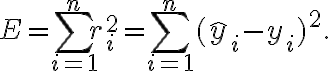
Setting the derivative of $E$ with respect to $m$ and $q$ to zero, the following formulas for $\hat{m}$ and $\hat{q}$ are found:

$\hat{m} = \dfrac{n \sum_{i=1}^n x_i y_i - \left(\sum_{i=1}^n x_i\right) \left(\sum_{i=1}^n y_i\right)} {n \sum_{i=1}^n x_i^2 - \left(\sum_{i=1}^n x_i\right)^2}$

$\hat{q} = \dfrac{\sum_{i=1}^n y_i - \hat{m} \sum_{i=1}^n x_i}{n}.$

Now that you have all the information you need to complete the task, use at least one of the two workspaces from previous lessons (Python or MATLAB) and write the code that gives the correct solution.

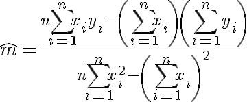
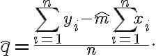
We just need to use the same code that we used during the lecture, extracting the BUI from the dataset with x = my_dataset["BUI"].values. The final Python code for the solution is the following:


import numpy as np
import matplotlib.pyplot as plt
import pandas as pd


def linear_regression(x, y):
    sum_x = np.sum(x)
    sum_y = np.sum(y)
    sum_xy = np.sum(x * y)
    sum_x2 = np.sum(x ** 2)

    n = len(x)
    numerator = n * sum_xy - sum_x * sum_y
    denominator = n * sum_x2 - sum_x ** 2
    m = numerator / denominator
    q = (sum_y - m * sum_x) / n

    return m, q


my_dataset = pd.read_csv('Algerian_forest_dataset.csv')
x = my_dataset['BUI'].values
y = my_dataset['FWI'].values
m, q = linear_regression(x, y)

print('Linear model results:')
print(f'Slope (m): {m}')
print(f'Y-intercept (q): {q}')

plt.figure(figsize=(16, 10))
plt.scatter(x, y, color='blue', alpha=0.5, label='Data points')
plt.plot(x, m * x + q, color='red', label='Regression line')

plt.xlabel('Temperature')
plt.ylabel('FWI')
plt.title('Linear Regression: FWI vs BUI')
plt.grid(True)
plt.legend()
plt.show()

We just need to use the same code that we used during the lecture, extracting the BUI from the dataset with x = my_dataset.BUI. The final Matlab code for the solution is the following:


my_dataset = readtable('Algerian_forest_dataset.csv');
x = my_dataset.BUI;
y = my_dataset.FWI;

[m, q] = my_linear_regression(x, y);

% Print results
disp('Linear model results:');
fprintf('Slope (m): %f\n', m);
fprintf('Y-intercept (q): %f\n', q);

figure;
scatter(x, y, 'blue', 'filled', 'MarkerFaceAlpha', 0.5);
hold on;
plot(x, m * x + q, 'red', 'LineWidth', 2);
xlabel('Temperature');
ylabel('FWI');
title('Linear Regression: FWI vs BUI');
grid on;
legend('Data points', 'Regression line');