Predict wildfire risk - Challenge 2: Compute the coefficient of determination R²
Task
Linear regression can always produce a fitting line given a set of data points  . However, how can we assess how well the regression line is fitting the available data? To answer, compute the coefficient of determination
  for temperature–FWI, RH–FWI, and BUI–FWI linear regressions in the Algerian forest dataset and evaluate which one of them has the best fit.
Below, we report the value of for each index:
- Coefficient of determination
forTemperature – FWI regression: .
. - Coefficient of determination
forRH – FWI regression: .
. - Coefficient of determination
forBUI – FWI regression: .
.
Among the three coefficients that we computed, the one associated to temperature is higher than the one relative to humidity: this could be interpreted as evidence that temperature plays a bigger role in influencing fire risk than relative humidity. However, such conclusion requires extensive knowledge of the specific field to be substantiated.
On the other hand, the BUI – FWI regression line coefficient is much higher than the other two, but the reason is actually very simple: BUI and FWI are both indices that quantify aspects of fire risk, and the BUI is one of the factors that is directly used in the computation of the FWI, so their correlation is naturally very high.
The coefficient of determination is defined as:
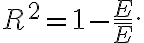
Where  is the sum of the squares of the residuals:
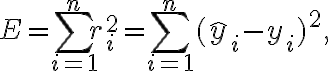
and  is the sum of the squared differences between the
  values and their mean
  :
:

In general, the lower the value of , the better the fit. However, the absolute value of depends on the scaling of the variables involved: scaling the dataset up will increase , even though intuitively the goodness of the fit should remain the same.
To circumvent this issue, we standardise the residuals, which requires computing a reference value. The quantity represents the variance intrinsic to the data and it can be seen as the "score" associated with a baseline regression model with  ,
,  , that is a model that always predicts the same value, equal to the mean of the dataset, no matter the input
  .
.
The quantity is always a value between 0 and 1: lower values indicate a poor fit, whereas higher ones indicate a good fit. The worst case  corresponds to the baseline model that we just discussed (
 ), while the best case scenario
  corresponds to a perfect fit, where the regression line interpolates all the data points without errors (
 ).
).
Finally, we remark that can also be interpreted as the fraction of explained variance of the model, i.e. how much of the intrinsic variance of the dataset is captured by the model versus how much of it is left unexplained.
To compute the coefficient of determination for our dataset, we need to compute and explicitly; to do this, we can use the concept of vectorized operations. In particular, we use the fact that adding a constant to a vector or multiplying it by a constant is treated in a vectorized manner, i.e. the operation is applied to all terms of the array.
We will define a function for each term: for we first need to compute the mean , while for the error we need the predicted values  .
.
def E_bar(y):
    y_bar = np.sum(y) / len(y)  # Mean of the dataset
    e_bar = np.sum((y - y_bar) ** 2)
    return e_bar


def E(x, y):
    m, q = linear_regression(x, y)
    y_hat = m * x + q  # Predicted values
    error = np.sum((y - y_hat) ** 2)
    return error


def R2(x, y):
    e_bar = E_bar(y)
    error = E(x, y)
    r_2 = 1 - error / e_bar
    return r_2
Note: the mean can also be computed directly with the np.mean function: y_bar = np.mean. Finally, we write one last function applying the definition of .
The final Python code for the solution is the following:
import numpy as np
import pandas as pd


def linear_regression(x, y):
    sum_x = np.sum(x)
    sum_y = np.sum(y)
    sum_xy = np.sum(x * y)
    sum_x2 = np.sum(x ** 2)

    n = len(x)
    numerator = n * sum_xy - sum_x * sum_y
    denominator = n * sum_x2 - sum_x ** 2
    m = numerator / denominator
    q = (sum_y - m * sum_x) / n

    return m, q


def E_bar(y):
    y_bar = np.sum(y) / len(y)  # Mean of the dataset
    e_bar = np.sum((y - y_bar) ** 2)
    return e_bar


def E(x, y):
    m, q = linear_regression(x, y)
    y_hat = m * x + q  # Predicted values
    error = np.sum((y - y_hat) ** 2)
    return error


def R2(x, y):
    e_bar = E_bar(y)
    error = E(x, y)
    r_2 = 1 - error / e_bar
    return r_2


my_dataset = pd.read_csv('Algerian_forest_dataset.csv')
Temperature = my_dataset['Temperature'].values
RH = my_dataset['RH'].values
BUI = my_dataset['BUI'].values
FWI = my_dataset['FWI'].values

r_2_Temperature = R2(Temperature, FWI)
r_2_RH = R2(RH, FWI)
r_2_BUI = R2(BUI, FWI)

print(f"Coefficient of determination for Temperature - FWI regression : {r_2_Temperature}")
print(f"Coefficient of determination for RH - FWI regression : {r_2_RH}")
print(f"Coefficient of determination for BUI - FWI regression : {r_2_BUI}")
To compute the coefficient of determination for our dataset, we need to compute and explicitly; to do this, we can use the concept of vectorized operations. In particular, adding a constant to a vector and multiplying it by a constant are treated in a vectorized manner, i.e. the operation is applied to all terms of the array. To specify that an operation should be vectorized, remember to put the dot . before it.
We will define a function for each term: for we first need to compute the mean , while for the error we need the predicted values .
function e_bar = E_bar(y)
    y_bar = sum(y) ./ length(y); % Mean of the dataset
    e_bar = sum((y - y_bar) .^ 2);
end


function error = E(x, y)
    [m, q] = my_linear_regression(x, y);
    y_hat = m .* x + q; % Predicted values
    error = sum((y - y_hat) .^ 2);
end


function r_2 = R2(x, y)
    e_bar = E_bar(y);
    error = E(x, y);
    r_2 = 1 - error / e_bar;
end
Note: the mean can also be computed directly with the mean function: y_bar = mean. Finally, we write one last function applying the definition of ;
.
The final Matlab code for the solution is the following:
function e_bar = E_bar(y)
    y_bar = sum(y) ./ length(y); % Mean of the dataset
    e_bar = sum((y - y_bar) .^ 2);
end


function error = E(x, y)
    [m, q] = my_linear_regression(x, y);
    y_hat = m .* x + q; % Predicted values
    error = sum((y - y_hat) .^ 2);
end


function r_2 = R2(x, y)
    e_bar = E_bar(y);
    error = E(x, y);
    r_2 = 1 - error / e_bar;
end


my_dataset = readtable('Algerian_forest_dataset.csv');
Temperature = my_dataset.Temperature;
RH = my_dataset.RH;
BUI = my_dataset.BUI;
FWI = my_dataset.FWI;

r_2_Temperature = R2(Temperature, FWI);
r_2_RH = R2(RH, FWI);
r_2_BUI = R2(BUI, FWI);

fprintf('Coefficient of determination for Temperature - FWI regression : %f\n', r_2_Temperature);
fprintf('Coefficient of determination for RH - FWI regression : %f\n', r_2_RH);
fprintf('Coefficient of determination for BUI - FWI regression : %f\n', r_2_BUI);