Computational Science & Computational Learning with Python and MATLAB: Blur a car plate - Challenge 3: New kernels

Task

Try applying the following two kernels to the car plate image. Can you guess what is their intended effect?

$K1 = \begin{bmatrix} -1 & 2 & -1\\ -1 & 2 & -1\\ -1 & 2 & -1 \end{bmatrix} \quad K2 = \begin{bmatrix} 0 & -1 & 0\\ -1 & 5 & -1\\ 0 & -1 & 0 \end{bmatrix}$

Figure 1: Left: Vertical edge detection. Right: sharpened image.

The kernel $K_{1}$ , which is a vertical edge detection kernel, produces a filtered image in which vertical lines correspond to high pixel values and thus appear white; on the other hand, horizontal edges and uniform regions produce a low (or even negative) value, and are displayed as black. If we used the transpose of this kernel, we would detect horizontal edges instead.

The convolution with the kernel $K_{2}$ sharpens the edges, making the contrast between the digits and the background of the car plate more apparent.

The first kernel is an edge detection filter. Intuitively, an edge is the “border” of an object, but how can we automatically find edges in an image? An edge can be described as an area characterized by a rapid change in color/intensity: inside the same object, pixel values will tend to be similar, forming uniform-looking region; on the other hand, if by moving in a particular direction we encounter a steep increase or decrease in image values, then we are likely on the border between two objects. The rate of change of intensity can be quantified by computing the derivatives of the image using finite differences.

Recall that the central finite difference formulas for estimating the first and second order derivatives of a real function are:

$f'(x) \approx \frac{f(x+h) - f(x-h)}{2h}, \quad f''(x) \approx \frac{f(x+h) - 2f(x) + f(x-h)}{h^2}$

Notice that the weights of one row of the kernel $[-1, 2, -1]$ are identical to the weights of the formula for $f''(x)$ (except with opposite sign)! This means that the convolution with this kernel is equivalent to computing the second partial derivative of the image in the horizontal direction. To better understand this, set the upper and lower rows of the kernel to zero:

$\left(A * \begin{bmatrix}0&0&0\\-1&2&-1\\0&0&0\end{bmatrix}\right)_{i,j} = -1 \times A_{i-1,j} + 2 \times A_{i,j} - 1 \times A_{i+1,j}$

The $h$ in the finite difference formula does not appear because it corresponds to the width of a pixel and is implicitly set to 1. Computing the horizontal derivative enables the detection of vertical edges, because an edge line is orthogonal to the direction with steepest intensity change, so the first kernel is actually a vertical edge detection kernel, to be more precise.

The second kernel is known as a sharpening kernel, because it enhances edges, making them “sharper”. The sharpening kernel can be decomposed as this sum:

$\begin{bmatrix} 0 & -1 & 0\\ -1 & 5 & -1\\ 0 & -1 & 0 \end{bmatrix} = \begin{bmatrix} 0 & 0 & 0\\ 0 & 1 & 0\\ 0 & 0 & 0 \end{bmatrix} + \begin{bmatrix} 0 & -1 & 0\\ -1 & 4 & -1\\ 0 & -1 & 0 \end{bmatrix} = K_I + K_E$

The first kernel $K_I$ is the identity kernel, that is 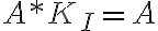$A * K_I = A$ . The second $K_E$ is once again an edge detection kernel, but instead of computing the derivative of the image only in the horizontal direction, it computes the laplacian, which is the sum of both second partial derivatives (horizontal and vertical):

$\Delta f(x,y) \;=\; \frac{\partial^2 f}{\partial x^2} + \frac{\partial^2 f}{\partial y^2} \;\approx\; \frac{1}{h^2}\Big(f(x+h,y) - 2f(x,y) + f(x-h,y)\Big) \;+\; \frac{1}{h^2}\Big(f(x,y+h) - 2f(x,y) + f(x,y-h)\Big)$ $=\; \frac{1}{h^2}\Big(f(x+h,y) + f(x,y+h) + f(x-h,y) + f(x,y-h) - 4f(x,y)\Big).$

$K_E$ highlights all edges, not only the vertical ones. Convolving the image with 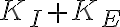$K_I + K_E$ is the equivalent to adding the detected edges back to the original image, which in practice means that the edges get amplified, making the image sharper.

Now that you have all the information you need to complete the task, use at least one of the two workspaces from previous lessons (Python or MATLAB) and write the code that gives the correct solution.

Since these two kernels are 3 by 3, we can reuse the code from the lecture, changing only the definition of the convolution kernel. In Python, we can initialize a two-dimensional array by using np.array and passing the elements as a nested list, that is a list of lists where each inner list corresponds to one row of the matrix.


K_edge_detection = np.array([[-1,  2, -1],
                             [-1,  2, -1],
                             [-1,  2, -1]])

K_sharpening = np.array([[ 0, -1,  0],
                         [-1,  5, -1],
                         [ 0, -1,  0]])

Then, we can just call im_filtering once for each of the kernels. The complete Python code is the following:


import numpy as np
from PIL import Image
from helper_functions import *

def local_convolution(A, K, i, j):
    v = 0
    for m in range(3):
        for n in range(3):
            v += A[i - 1 + m, j - 1 + n] * K[m, n]
    return v

def im_filtering(A, K):
    rows, cols = A.shape
    # Create an output matrix for the result
    R = np.zeros(shape=(rows - 2, cols - 2))

    for i in range(1, rows - 1):  # internal rows
        for j in range(1, cols - 1):  # internal columns
            R[i - 1, j - 1] = local_convolution(A, K, i, j)
    return R

# Load the image and convert it to gray scale
A = np.array(Image.open("plate.png").convert('L'))

# Create the convolution kernels
K_edge_detection = np.array(
    [[-1, 2, -1],
     [-1, 2, -1],
     [-1, 2, -1]]
)
K_sharpening = np.array(
    [[0, -1, 0],
     [-1, 5, -1],
     [0, -1, 0]]
)

# Padding
Ap = np.zeros((A.shape[0] + 2, A.shape[1] + 2))
Ap[1:-1, 1:-1] = A

R_edge_detection = im_filtering(Ap, K_edge_detection)
R_sharpening = im_filtering(Ap, K_sharpening)
compare_images(A, R_edge_detection)
compare_images(A, R_sharpening)

Since these two kernels are 3 by 3, we can reuse the code from the lecture, changing only the definition of the convolution kernel. In Matlab, we can initialize a matrix by listing its elements within square brackets [] separated by whitespace, with newlines denoting the beginning of a new row. Alternatively, it is possible to use a more explicit syntax and separate elements with colons and rows with semicolons.


K_edge_detection = [
    -1 2 -1
    -1 2 -1
    -1 2 -1
];
K_sharpening = [
    0 -1 0
    -1 5 -1
    0 -1 0
];

Then, we can just call im_filtering once for each of the kernels. The complete Matlab code is the following:


% Load the image and convert it to gray scale
A = double(rgb2gray(imread("plate.png")));

% Create the convolution kernels
K_edge_detection = [
    -1 2 -1
    -1 2 -1
    -1 2 -1
];
K_sharpening = [
    0 -1 0
    -1 5 -1
    0 -1 0
];

% Padding
Ap = zeros(size(A, 1) + 2, size(A, 2) + 2);
Ap(2:end - 1, 2:end - 1) = A;

R_edge_detection = im_filtering(Ap, K_edge_detection);
R_sharpening = im_filtering(Ap, K_sharpening);
compare_images(A, uint8(R_edge_detection))
compare_images(A, uint8(R_sharpening))