The radiotracer RTD method

The basic radiotracer methodology consists of accurate formulation of the Residence Time Distribution (RTD) experimental curve and its utilization for system analysis. RTD and the mean residence time (MRT) are generally used to determine the performance of the flow. MRT is the ratio between the volume and the flow rate in that volume, while its standard deviation (SD) characterizes the mixing rate: higher SD value corresponds to a higher mixing.
The major targets for radiotracer RTD methods are oil industries, petrochemical plants, mineral processing and wastewater treatment ponds. This system analysis supports the industrial reactor design, troubleshooting inspection, solving a wide range of problems. As example, a simple qualitative analysis of the shape of the RTD curve enables verification of the mixing. The principle of the radiotracer experiment is the common impulse-response method: injection of a tracer at the inlet of the system and recording the concentration-time curve at the outlet (Figure 1). The measurement of the count rate distribution (n_i) at the outlet of the system gives us the n_i values in cps or cpm at a specific time t.

Figure 1 - Principle of RTD method.

The RTD function is described by the so called exit age function, E(t):

$E(t) = \frac{C(t)}{\int_{0}^{\infty} C(t) dt}$

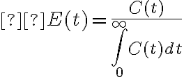
Where C(t) is the tracer concentration versus time at the outlet of the system. An example of E(t) function is represented in Figure 2 along with the relative MRT and SD parameters.

Figure 2 - E(t) function with MRT and SD parameters.

Proper corrections are applied to the data, required due to dead time of the detector, the background and due to the radioactive decay of the radiotracer during the experiment. The signal is then smoothed in order to decrease the fluctuations due to noise or counting statistic. If the end of the curve is missed for different reasons, data extrapolation can be performed.
Area normalization can be applied as a last step: it allows comparisons among different results (since it eliminates only the factors that affect the area, and not the shape). Moreover, it simplifies the calculation of the statistical parameters that characterize the curve, MRT and SD, as moments of the curve: 

$M_{i} =\int_{0}^{\infty} t^{i} E(t) dt$

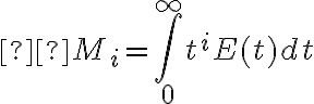
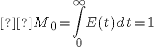
The zero^th moment is the area under the curve that, for a normalized curve, is equal to 1.

$M_{0}=\int_{0}^{\infty}E(t)dt=1$

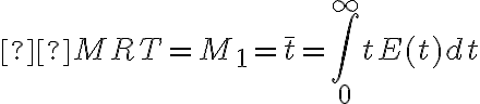
The MRT is equal to the first moment, i=1:

$MRT=M_{1}=\overline{t}=\int_{0}^{\infty}tE(t)dt$

The spread of the curve or SD (standard deviation) is indicated by σ. Its squared value σ², the variance, is given by:

$\sigma^{2}=M_{2}-M_{1}^{2}=\int_{0}^{\infty}(t-\overline{t})^{2}E(t)dt$

The experimental RTD curve is calculated from the count rate distribution measured at the system outlet, n_i (t), given in cps or cpm. Since the experimental data are recorded during consecutive time intervals of width Δt, the experimental E(t) function is reconstructed at the same time intervals, by normalizing the cpm:

$E_{i}=\frac{n_{i}(t)}{\sum_{i}n_{i}(t)\cdot\Delta t}$

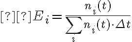
Where 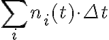$\sum_{i}n_{i}(t)\cdot\Delta t$ represent the total counts.
The momentum is calculated as:

$M_{0}=\sum_{i}E_{i}\Delta t=1$

$M_{1}=MRT=\overline{t}=\sum_{i}t_{i}E_{i}\Delta t$

$\sigma^{2}=\sum_{i}(t_{i}{}-{}\overline{t})^{2}E(t)\Delta t$

If we take as example the experimental data shown in Table 1 and in the relative graph Figure 3.

Table 1 - Radiotracer experimental data.

Figure 3 - Plot of the experimental data: cpm as a function of time.

Figure 4 - Plot of the cumulative experimental data: cpm as a function of time.

In the example, total counts are 145000.

$MRT= 20.05 min$

The spread of RTD is the standard deviation of the distribution, the second momentum.

$\sigma^{2}=68.19$

$\sigma=8.25$