Control a robotic arm - Challenge 1: Plot the Objective function J
Task
Try to run the Gradient Descent algorithm saving the value of the objective function  at each iteration. At the end of the loop, plot as a function of the iteration counter. Consider
  ,
,  ,
, 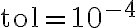 ,
,  , and initial conditions
  . Comment the results.
The figure below shows the squared distance of the robot arm tip to the target as a function of Gradient Descent iterations. We can see that initially the objective function decreases quite fast, with a decrease of the order of 100 per iteration, while later this rate slows down to around  per iteration, until the algorithm stops because we have reached the required tolerance .

Figure 1: Squared distance of the robot arm tip to the target as a function of Gradient Descent iteration, shown with logarithmic y axis.
Gradient Descent is an iterative algorithm used to solve (approximately) a minimization problem:
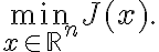
This is done by taking an initial guess  and updating it by moving in the direction opposite to the gradient of :

The main idea behind the algorithm is that the gradient of a function corresponds to the direction of its greatest increase, so moving in the opposite direction means decreasing the objective function. The magnitude of the update depends on the parameter  , which is called learning rate or step size.
In our robot arm example, the objective function is the squared distance between the robot tip  and the target point
 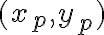 :
:

At each iteration we take a step that is proportional to the gradient of , so the steepest the gradient, the larger the step and thus the decrease. Near the minimum of the objective function , the function is much "flatter", i.e. the gradient magnitude is low, and so the convergence is slower.
The code for the algorithm is the same as the one seen in the lecture, we just have to modify it slightly to store values of .
However, since Gradient Descent can take a different number of iterations to converge depending on the parameters that we use, we do not know a priori how many values we will get. This means that we cannot allocate a list "statically" with dp = N * [0] like we did before: we have to instead grow the list dynamically while the algorithm progresses. To do this, we can use the append method, which takes as input an object and inserts it at the end of the list, increasing its length by one, as in the following example:
a = [2, 3] # List has two
            elements
a.append(4) # Now the list has 3 elements:
[2, 3, 4]
In our code, at the start of the algorithm we initialize an empty list with values = []. Then, at each iteration of the while loop, we append the new value: values.append(Jval).
To better visualize the sequence, instead of plt.plot we will use plt.semilogy, which plots the data using a logarithmic y axis; this is useful because the values of will span across multiple orders of magnitude. Since we want to plot the values against the number of iterations, we can pass values as the only argument to plt.semilogy; in that case the corresponding x value of a given entry of a vector will just be its index in the vector, which is exactly what we need. The final Python code for the solution is the following:
from math import sin, cos
from matplotlib import pyplot as plt

# Input parameters
L1 = 1      # length of arm1
L2 = 1.5    # length of arm2
theta = [2.5, 2.7]  # initial angles
tol = 0.0001        # tolerance
alpha = 0.1         # learning rate
Niter = 100         # max iterations

xp = [0.75, -1]

# Compute tip robot position
def robot_position(theta, L1, L2):
    theta1, theta2 = theta
    x = L1 * cos(theta1) + L2 * cos(theta2)
    y = L1 * sin(theta1) + L2 * sin(theta2)
    return [x, y]

# Evaluation of J
def J(theta, xp, L1, L2):
    [x, y] = robot_position(theta, L1, L2)
    Jval = (x - xp[0]) ** 2 + (y - xp[1]) ** 2
    return Jval

# Evaluation of grad(J)
def grad_J(theta, xp, L1, L2):
    [x, y] = robot_position(theta, L1, L2)

    dx_dt1 = -L1 * sin(theta[0])
    dx_dt2 = -L2 * sin(theta[1])
    dy_dt1 = L1 * cos(theta[0])
    dy_dt2 = L2 * cos(theta[1])

    dJ_dx = 2 * (x - xp[0])
    dJ_dy = 2 * (y - xp[1])

    DJ_dt1 = dJ_dx * dx_dt1 + dJ_dy * dy_dt1
    DJ_dt2 = dJ_dx * dx_dt2 + dJ_dy * dy_dt2

    return [DJ_dt1, DJ_dt2]

plt.figure(figsize=(10, 5))

values = []
i = 1
while i <= Niter:
    # Gradient of the objective function
    grad = grad_J(theta, xp, L1, L2)
    # Update theta with gradient
    theta[0] -= alpha * grad[0]
    theta[1] -= alpha * grad[1]
    # Compute the current value
    Jval = J(theta, xp, L1, L2)
    values.append(Jval)
    # Check for convergence
    if Jval < tol:
        print(f"Converged after {i} iterations.")
        break
    i = i + 1

plt.semilogy(values, marker='o', markersize=3)

plt.xlabel("Iterations")
plt.ylabel("J")
plt.title("Objective function values")
plt.grid()
plt.show()
The code for the algorithm is the same as the one seen in the lecture, we just have to modify it slightly to store the distances.
Since the number of iterations needed by Gradient Descent to converge is not known a priori, we cannot use zeros(N) like before to store the distance values; instead we need to grow a vector dynamically while the algorithm progresses. Matlab allows us to do this by simply accessing the corresponding index of the vector and assigning a value to it: if the vector is shorter than the index that we access, the corresponding element will be created in that moment (and any other intermediate values will be filled with zeros), like in this example:
a = [2, 3]; % Vector has 2
            elements
a(5) = 4; % Now it has 5 elements: a = [2,
3, 0, 0, 4]
So, at the start of the algorithm we initialize an empty vector with values = []; and then add to it the computed distances with values(i) = Jval; at each while loop iteration.
Another way of appending elements that is more explicit in its syntax is concatenation:
a = [2, 3]; % Vector has 2
            elements
a = [a, 4]; % a is concatenated with 4, so
a = [2, 3, 4]
To better visualize the sequence, instead of plot we will use semilogy, which plots the data using a logarithmic y axis; this is useful because the values of will span across multiple orders of magnitude. Since we want to plot the values against the number of iterations, we can pass values as the only argument to semilogy; in that case the x value corresponding to a given entry of the vector will just be its index in the vector, which is exactly what we need. The final Matlab code for the solution is the following:
% Input parameters
L1 = 1;      % length of arm1
L2 = 1.5;    % length of arm2
theta = [2.5 2.7];  % initial angles
tol = 0.0001;      % tolerance
alpha = 0.1;       % learning rate
Niter = 100;       % max iteration number

xp = [0.75, -1];

% Compute tip robot position
function [x, y] = robot_position(theta, L1, L2)
    x = L1 * cos(theta(1)) + L2 * cos(theta(2));
    y = L1 * sin(theta(1)) + L2 * sin(theta(2));
end

% Evaluation of J
function Jval = J(theta, xp, L1, L2)
    [x, y] = robot_position(theta, L1, L2);
    Jval = (x - xp(1)) ^ 2 + (y - xp(2)) ^ 2;
end

% Evaluation of grad(J)
function grad = grad_J(theta, xp, L1, L2)
    [x, y] = robot_position(theta, L1, L2);

    dx_dt1 = -L1 * sin(theta(1));
    dx_dt2 = -L2 * sin(theta(2));
    dy_dt1 = L1 * cos(theta(1));
    dy_dt2 = L2 * cos(theta(2));

    dJ_dx = 2 * (x - xp(1));
    dJ_dy = 2 * (y - xp(2));

    DJ_dt1 = dJ_dx * dx_dt1 + dJ_dy * dy_dt1;
    DJ_dt2 = dJ_dx * dx_dt2 + dJ_dy * dy_dt2;

    grad = [DJ_dt1, DJ_dt2];
end

% Create figure for plotting
figure()

% Gradient Descent Method
values = [];
i = 1;
while i <= Niter
    % Gradient of the objective function
    grad = grad_J(theta, xp, L1, L2);
    % Update theta with gradient
    theta = theta - alpha * grad;
    % Compute the current value
    Jval = J(theta, xp, L1, L2);
    values(i) = Jval;
    % Check for convergence
    if Jval < tol
        fprintf('Converged after %d iterations.\n', i)
        break
    end
    i = i + 1;
end

semilogy(values, '-o', 'markersize', 3)
grid on
xlabel('i')
ylabel('J')