Control a robotic arm - Challenge 2: Unreachable target
Task
Consider as a target the point  and run the Gradient Descent algorithm with these data:
  ,
, 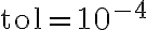 ,
,  , and initial conditions
  . Plot the value of
  as a function of the iteration counter and represent the final robot configuration. What do you observe?
The following figure shows the squared distance of the robot arm tip to the target as a function of Gradient Descent iterations with a logarithmic y axis.

Figure 1: Squared distance of the robot arm tip to the target as a function of Gradient Descent iterations, shown with logarithmic y axis.
As highlighted, the sum of the length of the robot arms is  , while the distance of the target from the base is
  , so the point is not reachable by the robot tip. However, the Gradient Descent algorithm does not really care about this: the distance between the robot tip and the target is minimized, which means that the robot stretches out in its direction without actually ever reaching it. Since this minimum distance is much greater than the tolerance that we fixed, the stop criterion will never be satisfied and the algorithms runs for the maximum number of iterations . The final robot configuration is shown in the following figure:

Figure 2: Final robot configuration in the case of an unreachable target.
The Gradient Descent will minimize the squared distance between the robot tip  and the target point
 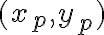 :
:

If the target point is reachable by the robot tip the minimum value of is zero, but if the point is "too far" the minimum of the squared distance will be positive.
The code for the algorithm is analogous to Challenge 1, with a different target point and the addition of the plotting of the robot final configuration. Therefore, we need to import the function plot_robot_arm from my_functions. The final Python code for the solution is the following:
from math import sin, cos
from matplotlib import pyplot as plt
from my_functions import plot_robot_arm

# Input parameters
L1 = 1       # length of arm1
L2 = 1.5     # length of arm2
theta = [2.5, 2.7]  # initial angles
tol = 0.0001        # tolerance
alpha = 0.1         # learning rate
Niter = 100         # max iterations

xp = [2, 2.5]

# Compute tip robot position
def robot_position(theta, L1, L2):
    theta1, theta2 = theta
    x = L1 * cos(theta1) + L2 * cos(theta2)
    y = L1 * sin(theta1) + L2 * sin(theta2)
    return [x, y]

# Evaluation of J
def J(theta, xp, L1, L2):
    [x, y] = robot_position(theta, L1, L2)
    Jval = (x - xp[0]) ** 2 + (y - xp[1]) ** 2
    return Jval

# Evaluation of Grad(J)
def grad_J(theta, xp, L1, L2):
    [x, y] = robot_position(theta, L1, L2)

    dx_dt1 = -L1 * sin(theta[0])
    dx_dt2 = -L2 * sin(theta[1])
    dy_dt1 = L1 * cos(theta[0])
    dy_dt2 = L2 * cos(theta[1])

    dJ_dx = 2 * (x - xp[0])
    dJ_dy = 2 * (y - xp[1])

    DJ_dt1 = dJ_dx * dx_dt1 + dJ_dy * dy_dt1
    DJ_dt2 = dJ_dx * dx_dt2 + dJ_dy * dy_dt2

    return [DJ_dt1, DJ_dt2]

values = []
i = 1
while i <= Niter:
    # Gradient of the objective function
    grad = grad_J(theta, xp, L1, L2)
    # Update theta with gradient
    theta[0] -= alpha * grad[0]
    theta[1] -= alpha * grad[1]
    # Compute the current value
    Jval = J(theta, xp, L1, L2)
    values.append(Jval)
    # Check for convergence
    if Jval < tol:
        print(f"Converged after {i} iterations.")
        break
    i = i + 1

plt.figure(figsize=(10, 5))
plt.semilogy(values, marker='o', markersize=3)
plt.xlabel("Iterations")
plt.ylabel("J")
plt.title("Objective function values")
plt.grid()
plt.show()

plt.figure(figsize=(10, 5))
plot_robot_arm(theta, xp, [L1, L2])
The code for the algorithm is analogous to Challenge 1, with a different target point and the addition of the plotting of the robot final configuration. Therefore, we need the function plot_robot_arm, so we need to tell Matlab "where it is", using addpath. The final Matlab code for the solution is the following:
% Input parameters
L1 = 1;      % length of arm1
L2 = 1.5;    % length of arm2
theta = [2.5 2.7];  % initial angles
tol = 0.0001;      % tolerance
alpha = 0.1;       % learning rate
Niter = 100;       % max iteration number

xp = [2, 2.5];

% Compute tip robot position
function [x, y] = robot_position(theta, L1, L2)
    x = L1 * cos(theta(1)) + L2 * cos(theta(2));
    y = L1 * sin(theta(1)) + L2 * sin(theta(2));
end

% Evaluation of J
function Jval = J(theta, xp, L1, L2)
    [x, y] = robot_position(theta, L1, L2);
    Jval = (x - xp(1)) ^ 2 + (y - xp(2)) ^ 2;
end

% Evaluation of grad(J)
function grad = grad_J(theta, xp, L1, L2)
    [x, y] = robot_position(theta, L1, L2);

    dx_dt1 = -L1 * sin(theta(1));
    dx_dt2 = -L2 * sin(theta(2));
    dy_dt1 = L1 * cos(theta(1));
    dy_dt2 = L2 * cos(theta(2));

    dJ_dx = 2 * (x - xp(1));
    dJ_dy = 2 * (y - xp(2));

    DJ_dt1 = dJ_dx * dx_dt1 + dJ_dy * dy_dt1;
    DJ_dt2 = dJ_dx * dx_dt2 + dJ_dy * dy_dt2;

    grad = [DJ_dt1, DJ_dt2];
end

% Create figure for plotting
figure()

% Gradient Descent Method
values = [];
i = 1;
while i <= Niter
    % Gradient of the objective function
    grad = grad_J(theta, xp, L1, L2);
    % Update theta with gradient
    theta = theta - alpha * grad;
    % Compute the current value
    Jval = J(theta, xp, L1, L2);
    values(i) = Jval;
    % Check for convergence
    if Jval < tol
        fprintf('Converged after %d iterations.\n', i)
        break
    end
    i = i + 1;
end

semilogy(values, '-o', 'markersize', 3)
grid on
xlabel('i')
ylabel('J')

figure
plot_robot_arm(theta, xp, [L1, L2])